Envelopes of Solids of Revolution

Flank milling is a manufacturing process in which material is removed from the workpiece using a cutter rotating at high speed. Since the cutter rotates much faster than the feed rate of the tool, the cutter can be thought of as a solid of revolution, and the envelope swept by this solid becomes the final surface of the workpiece.

Numerous books on differential geometry delve into the topic of envelopes, such as (Kreyszig, 1991, Section 85). In our paper (Ponce-Vanegas et al., 2023) [link to paper] we explore the impact of both the regularity of the profile and the trajectory of the tool on the smoothness of the envelope.

The profiles and trajectories of tools are designed using splines, and these lose smoothness at the knots, so it is important to understand the effect of this loss of smoothness on the swept envelope. In our paper we illustrate these effects with pictures of envelopes generated under various conditions. The purpose of this post is to show how to create one of these pictures, specifically Figure 9 in our paper.

Warning: since this post is based on (Ponce-Vanegas et al., 2023), I will use the notation and concepts in it without further notice.

Figure 9 was rendered using POV-Ray , and the parameterization of the different geometrical objects was done with Matlab. The code has been uploaded to BCAM’s GitLab , and from now on I will refer to the files as found there.

Note: The code was tested only in Ubuntu.

Matlab Code

The directory src contains the basic program to generate envelopes. There are three files, one for each class: Tool, RigidMotion and Envelope. All these classes are used in Example/C1_Envelope.m for Figure 9.

The Tool class

First, we define in C1_Envelope.m the profile of the tool using spmak:

L = 0.8;
pfl = spmak([-L/2 -L/2 -L/2 0 L/2 L/2 L/2], ...
    [0.1 0.1 0.25 0.25]);

This is a B-spline of order 3 representing a tool of length L, so the profile of the tool is $C^1$, and $0$ is the point where smoothness is lost. To create an instance of Tool we write:

tl = Tool(pfl);

The class Tool has the method plot, which is invoked using tl.plot(k), to visualize the $k$-derivative of the profile of the tool. For instance, using tl.plot(2) the discontinuity at $0$ is evident.

The method plot also allows us to create files which can be then read by POV-Ray. tl.plot(povray=true) will save a file called tool.txt, which contains the instructions POV-Ray needs to render the tool using lathe.

The RigidMotion class

We assume that the tool is a solid of revolution around the axis $x_3$. We can describe the motion of the tool with a rigid motion $E$ as

\[E(t)\bold{y} := R(t)\bold{x} + \bold{a}(t),\]

where $R \in SO(3)$ is a rotation, $\bold{a}$ is a translation, and $t$ is time; here, $t$ does not refer to the physical time but to a progress parameter. Nothing is lost if we assume that $a_2 = t$, because we can always use a rigid motion and a time re-parameterization to enforce this condition. In fact, the code was only tested under this assumptions, and a very different choice may affect the performance of the code.

In general, to specify a rotation we need 3 parameters, but because of the symmetry of the tool this number goes down to 2. For the RigidMotion class we chose the parameterization

\[\begin{gather} R(\theta,\varphi) = U(\theta)\,V(\varphi), \\ \\ U(\theta) = \begin{pmatrix} 1 & 0 & 0 \\ 0 & \cos(\theta) & \sin(\theta) \\ 0 & -\sin(\theta) & \cos(\theta) \end{pmatrix} \quad \text{and} \quad V(\varphi) = \begin{pmatrix} \cos(\varphi) & 0 & \sin(\varphi) \\ 0 & 1 & 0 \\ -\sin(\varphi) & 0 & \cos(\varphi) \end{pmatrix}, \end{gather}\]

where $\theta \in [-\pi/2, \pi/2)$, and $\varphi \in [-\pi/2, \pi/2)$. Hence, the motion of the tool is completely determined by $\theta$, $\varphi$, and $\bold{a}$.

rotation

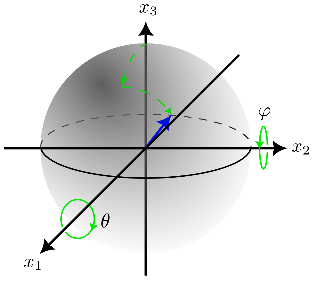
A rotation of a solid of revolution can be seen as a vector in the unit sphere. If $\theta$ and $\varphi$ are small, then $R\bold{e}_3 \approx (\varphi, \theta, 1)$.

For Figure 9 we used the trajectory

theta = spmak([0 1 2 2 2], 0.25*pi*[-0.4 0.3]);
phi = spmak([0 1 2 2 2], 0.25*pi*[-0.5 -0.1]);
a1 = spmak([0 1 2 2 2], [0.5 -0.2]);
a2 = spmak([0 2 2], 2);
a3 = spmak([0 1 2 2 2], [-0.6 -0.8]);

Now we can create an instance of RigidMotion:

rm = RigidMotion(theta, phi, a1, a2, a3);

RigidMotion has the method plot_rotation, which plots the curve $R(t)\bold{e}_3$ in the unit sphere. Also, the method rm.exp_povray(2) creates a file named rotation_2.000.txt, which POV-Ray can read to place the tool at the end of the envelope at time $t = 2$.

The Envelope class

This is the more complex class, and I explain here only what is strictly necessary; at the end of this post I give more details. To instantiate the class we need a tool and a rigid motion:

e = Envelope(tl, rm);

Since the envelope tends to be singular along the edge of regression (Ponce-Vanegas et al., 2023)[Theorem 3], we want to rule out its presence by checking that $\partial_t^2 G$ does not change sign. For that, we can use e.plot_Gtt(2^6 + 1, 2^6 + 1); and inspect the plot; the arguments of plot_Gtt are the number of subdivisions of the time interval and tool length, respectively.

To see the envelope swept by tl subject to the motion rm, type

e.plot_envelope(2^5 + 1, 2^5 + 1);
axis equal;

Since our goal is to visualize the envelope in POV-Ray, we can use e.plot_envelope(2^5 + 1, 2^5 + 1, povray=true); to generate a file called envelope.txt, which saves the points of the envelope and the normal vectors to each of them so that POV-Ray can read them as smooth triangles in a mesh.

We can also plot the characteristic curves and streamlines on the envelope. For that, type hold on to hold the plot of the envelope, and then type e.plot_characteristic(1, 2^7 + 1); and e.plot_time_curves(0, 2^7 + 1);. We can see now the characteristic curve at time $t = 1$, and the streamline at tool height $l = 0$; both methods also have a povray keyword argument to generate files which POV-Ray can read. We emphasize these curves because smoothness is lost along them.

POV-Ray Code

The goal of this section is to generate the envelope defined in the previous section. The code is in the file Example/C1_Regular.pov, and the image is rendered typing in the terminal povray C1_Regular.pov MySettings.ini.

rotation

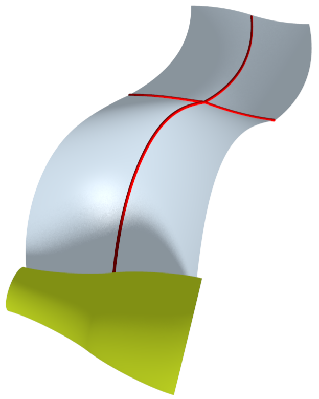
Envelope with the tool (green) depicted at the final time.

Basic information about the placement of the camera and the light source in POV-Ray can be found here. Recall that in the previous section we generated the files:

tool.txt
envelope.txt
rotation_2.000.txt
char_100_whole.txt
time_curve_whole.txt

which must be saved in the directory that contains C1_Regular.pov.

To endow the tool and envelope with a shiny look, we defined the finish:

#declare MyFinish = finish { 
  ambient .6
  diffuse .6
  phong 0.4
  phong_size 40
}

Following the C++ tradition, we declared the objects before using them. We declare the tool as a lathe object:

#declare Tool = union {
  lathe {
    bezier_spline
    #include "tool.txt"
    texture{
      pigment { color rgbf<94/255,119/255,3/255, 0> }
      finish { MyFinish }
    }
    sturm
  }
}

We needed the sturm keyword to avoid oddities in the tool.

The envelope is declared as a mesh:

#declare Envelope = mesh {
  #include "envelope.txt"
}

The file envelope.txt uses the macro smooth_quad, which is defined in Example/MyMacros.inc. This macro merges two smooth triangles into a “smooth square”.

We include the following code at the end of C1_Regular.pov to place the tool and the envelope in the picture:

object {
  Envelope
  texture {
    pigment { color rgb<106/255,125/255,142/255> }
    finish { MyFinish }
  }
}

object {
  Tool
  #include "rotation_2.000.txt"
}

The characteristic curve at time $t=1$ and the streamline at tool height $l=0$ are included with the following code:

#include "char_100_whole.txt"
curve(-0.4, 0.4, 8e-3, 1e-3, <255/255,0/255,0/255>)

#include "time_curve_whole.txt"
curve(0, 2, 8e-3, 1e-3, <255/255,0/255,0/255>)

The macro curve is defined in MyMacros.inc.

About the Envelope class

Other methods:

contact_lin_sys: computes the coefficients of the linear system in (Ponce-Vanegas et al., 2023) Eq. (8).

The arguments Qt and Ql are optional, and are used to speed up some computations. For instance, in the method plot_envelope the envelope is computed at the points $(t_i, l_j)$, for $i = 1,\ldots, N_t$ and $j = 1, \ldots, N_l$, so we can save resources computing some quantities only once when they only depend on time or tool height.

dir_contact: computes the direction vector in (Ponce-Vanegas et al., 2023) Eq. (9).

surface: computes the image of $(t, l)$ in the envelope.

References

Kreyszig, E. (1991). Differential geometry (p. xiv+352). Dover Publications, Inc., New York.
Ponce-Vanegas, F., Bizzarri, M., & Bartoň, M. (2023). On C0 and C1 continuity of envelopes of rotational solids and its application to 5-axis CNC machining. Computer Aided Geometric Design, 102245. https://doi.org/10.1016/j.cagd.2023.102245